
Simple Continuum Calibration
1. Data overview
Project 2016.1.00434.S (PI Smail) "Unlocking our understanding of submm galaxies with ALMA identifications for >1000 SMGs" continuum snapshots at Band 7. This Science Goal contains 44 targets, plus one each bandpass, flux scale and phase-reference calibrators. Originally the data were calibrated by the pipeline but for this workshop a manual script is provided to illustrate the calibration steps.
We provide input files which you can get as below in advance or from a USB drive on the day
wget -c http://almanas.jb.man.ac.uk/alma/Web/Meetings/2018/DurhamSchool/uid___A002_Xba4d35_Xb297.ms.split.tarwget -c http://almanas.jb.man.ac.uk/alma/Web/Meetings/2018/DurhamSchool/uid___A002_Xba4d35_Xb297.ms.scriptForCalibration.py
Extract the measurement set: (about 2.6 G)
tar -xvf uid___A002_Xba4d35_Xb297.ms.split.tar
uid___A002_Xba4d35_Xb297.ms.scriptForCalibration.py is a python script which you can open in a suitable viewer (e.g. emacs)
The steps 0-8 in the script have already been run, as the initial data volume is about 40 G and normally there is no need to change the standard parameter settings, the more interesting are described for information.
2. Initial and instrumental calibration, flagging etc.
The data were converted from ASDM (ALMA Science Data Model) format to Measurement Set in step 0:
mystep='0'
if os.path.exists('uid___A002_Xba4d35_Xb297.ms') == False:    # only import if ms does not already exist
importasdm('uid___A002_Xba4d35_Xb297',
            asis='Antenna Station Receiver Source CalAtmosphere CalWVR CorrelatorMode SBSummary',
                               # import metadata tables such as antenna position list
            bdfflags=True,     # import table of online-generated flags
            lazy=False, process_caldevice=False)
Step 1 is a correction of metadata (not in fact needed for these data).
Step 2 in the script produces a text listing of the MS
os.system('rm -rf uid___A002_Xba4d35_Xb297.ms.listobs') # remove any old file of this name
listobs(vis = 'uid___A002_Xba4d35_Xb297.ms',
        listfile = 'uid___A002_Xba4d35_Xb297.ms.listobs')
Step 3 applies known flags, such as spectral windows used only for online quality checks and times when the telescope are slewing between fields.
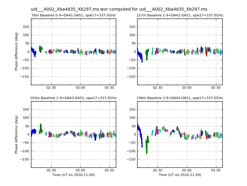
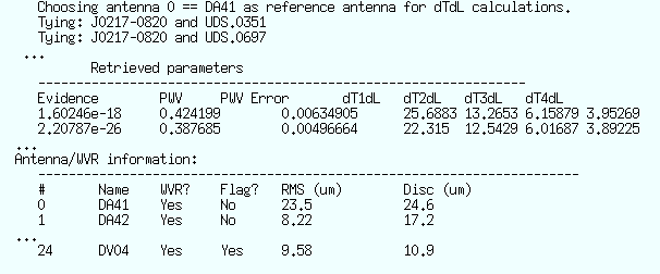
Steps 4 and 5 use the Water Vapour Radiometry (WVR) and System Temperature (Tsys) measurements to generate calibration tables. A shortcut is used to produce plots only possible with a special library, so these are provided ready-made; the self-cal tutorial will show how to make plots more simply. There is also a wvrgcal log file which lists the PWV measurements, here around 0.38-0.45 mm.
mysteps=[3,4,5,6]
 execfile('uid___A002_Xba4d35_Xb297.ms.scriptForCalibration.py')
The script (or pipeline commands) are generated with access to ALMA parameters covering the observation period. This is used to check for antenna position updates, which are listed in the script and Step 6 writes these to the antenna position correction table.
These correction tables are then applied to the data in Step 7. Task applycal is run separately for each calibration source and for all targets together, as they are all close on the sky and share the same calibration. This is derived from one target (34) for Tsys; for wvr this has already been interpolated to the targets from the phase reference corrections by task wvrgcal. tsysmap does not change anything here but it is used if TDM corrections are applied to narrow FDM spw. Here is the target example.
applycal(vis = 'uid___A002_Xba4d35_Xb297.ms',
    field = '4~48',                   # all the target fields
    spw = '17,19,21,23',              # The science spw
    gaintable = ['uid___A002_Xba4d35_Xb297.ms.tsys', 'uid___A002_Xba4d35_Xb297.ms.wvr', 'uid___A002_Xba4d35_Xb297.ms.antpos'],
                                      # The Tsys, WVR and antenna pos. correction tables
    gainfield = ['34', '', ''],       # Use the Tsys correction from field 34.
    interp = 'linear,linear',
    spwmap = [tsysmap,[],[]],
    calwt = True,
    flagbackup = False)
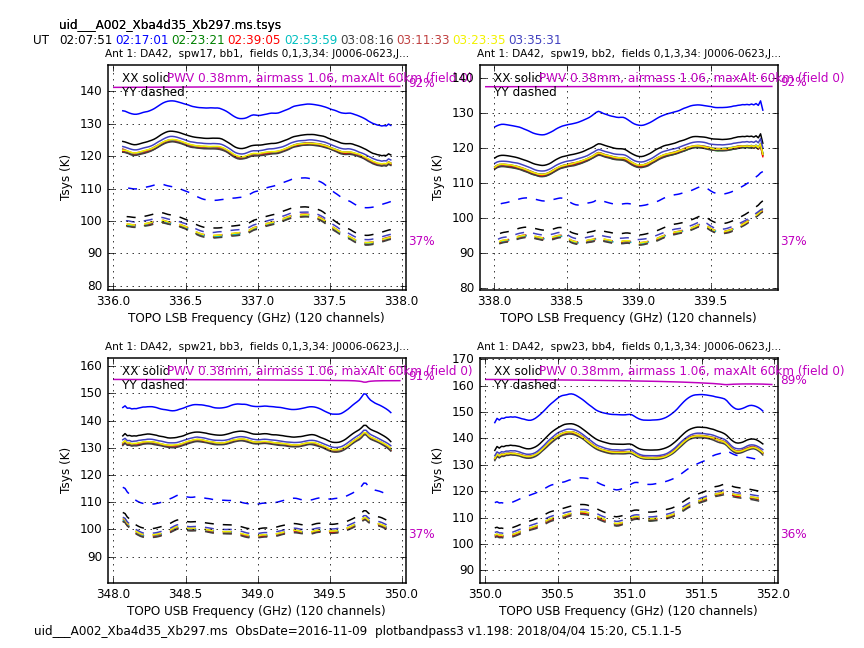
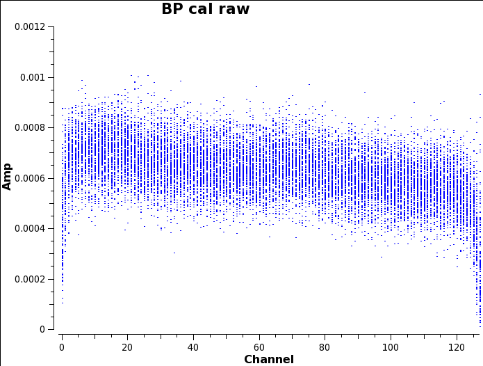
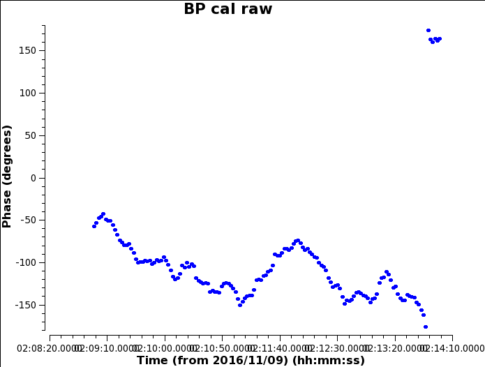
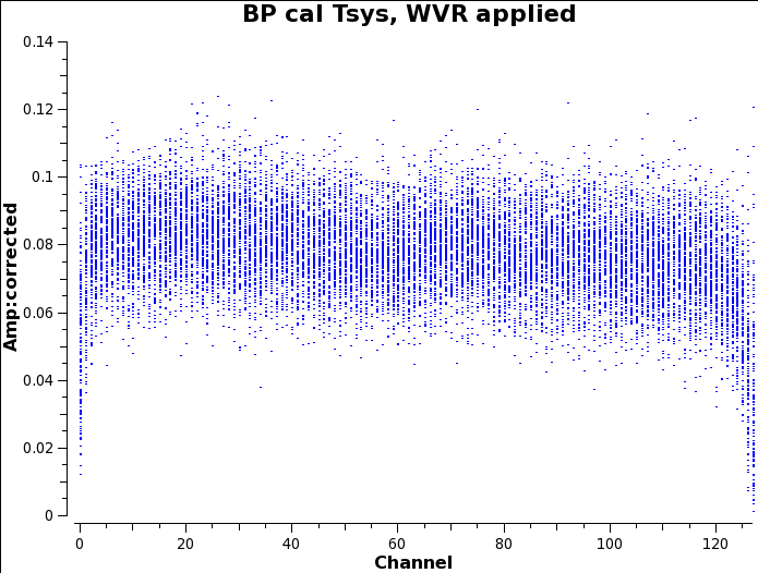
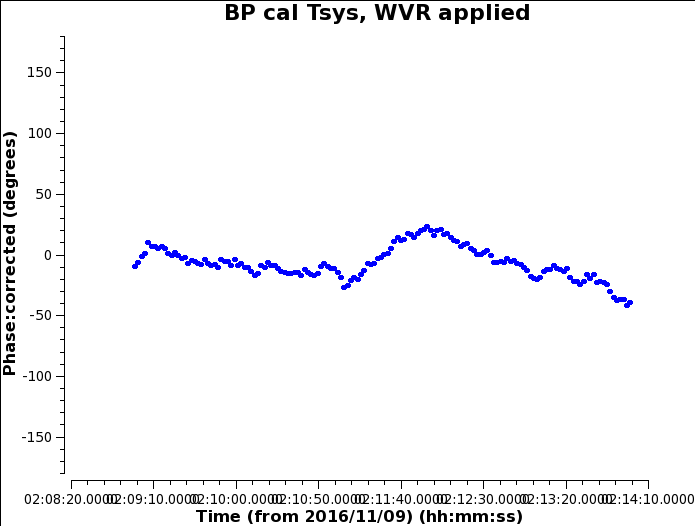
The plots below show the bandpass calibrator amplitude as a function of channel and phase as a function of time, before and after applying Tsys and WVR corrections (one baseline, one spw, some averaging)
If doing these stages manually, one would check the calibration table plots and the data for the calibration sources, and, all being well, in Step 8 split out the science spectral windows.
The output is uid___A002_Xba4d35_Xb297.ms.split
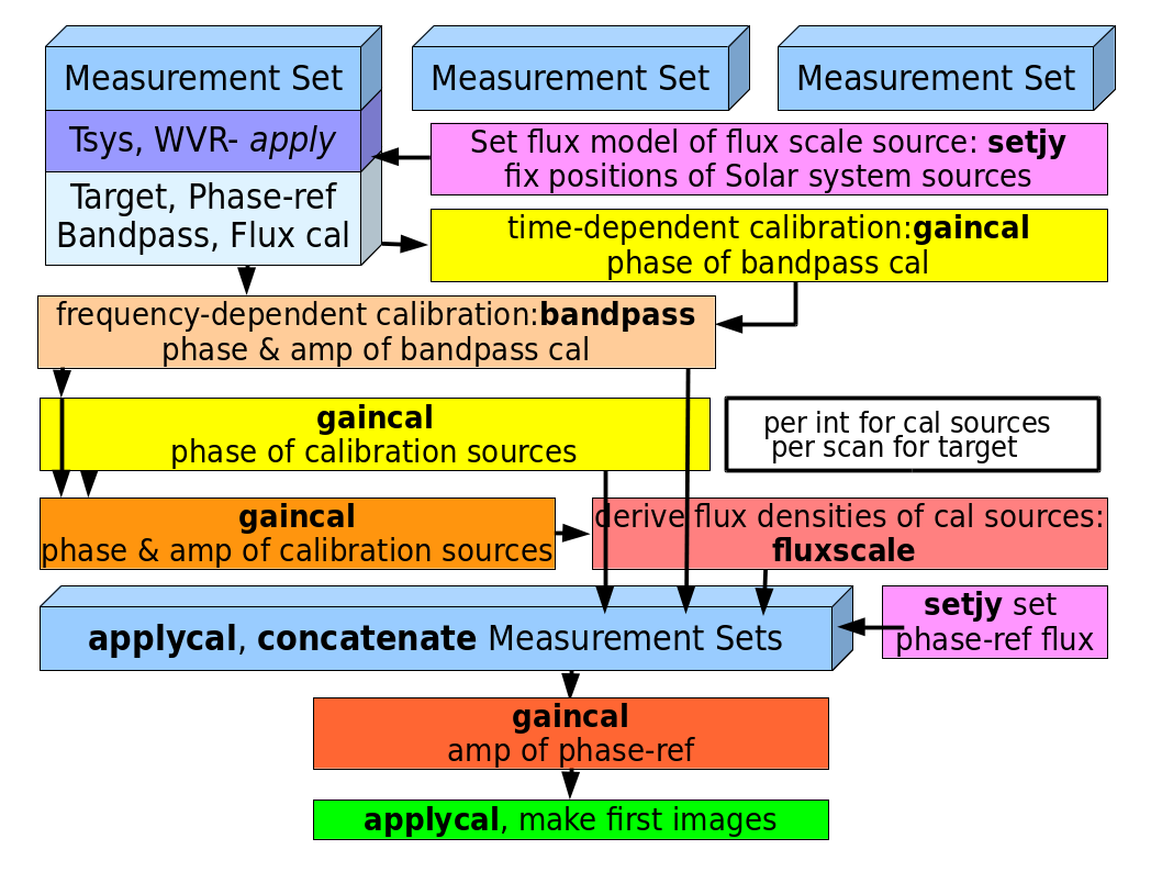
3. Derive and apply bandpass, flux-scale and phase reference calibration
Working in a directory which is not part of your CASA installation, containing the input files listed in Sec. 1. Start CASA. How you do this depends on your preferences and o/s but on linux SL6, if the installation is in your home area, for example:
~/casa-release-5.4.0-68.el6/bin/casa
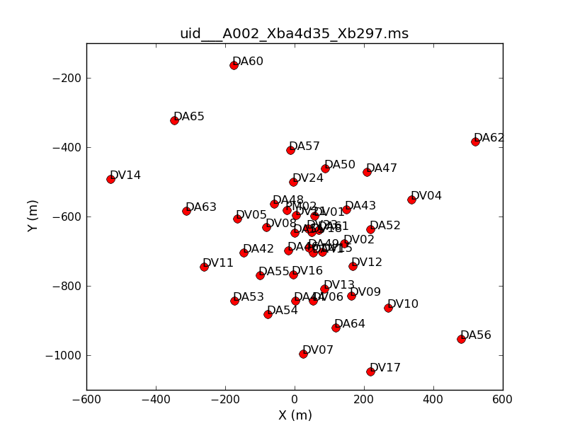
Then at the CASA prompt, type commands in red. First, off-script, examine the antenna distribution. this is an interactive way to enter commands so that you can check each parameter:
default plotants
 inp # see the inputs
 vis='uid___A002_Xba4d35_Xb297.ms.split' # no comma if parameters entered like this
figfile= 'uid___A002_Xba4d35_Xb297.plotants.png'
 inp # check again
 plotants # execute the task
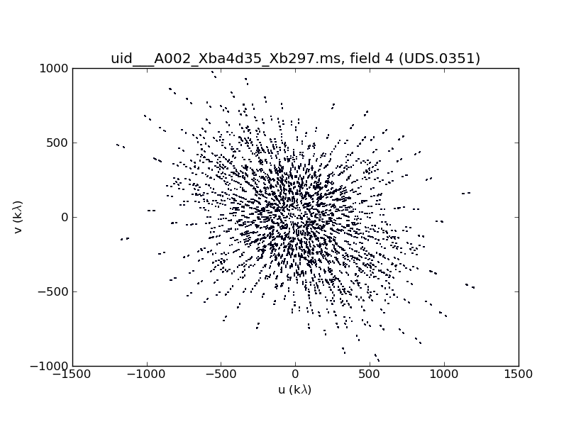
NB Don't do plotuv if you have a slow computer!
default plotuv
inp
 vis='uid___A002_Xba4d35_Xb297.ms.split'
 field='UDS.0351' # just plot one target field
 maxnpts=5000000
figfile= 'uid___A002_Xba4d35_Xb297.UDS.0351_plotuv.png'
inp
plotuv
Inspect in plotms interactively.
Look in the script to find the refant
Use listobs to identify science spw (here, 17,19,21,23)
Select bandpass calibrator field 0
Average channels, colourise by baseline (Display)
Plot amp v. time, all baselines to refant, iterate over spw (Page)
Plotms shows that one antenna has low gains. Mark and Locate reveal that this is DV04
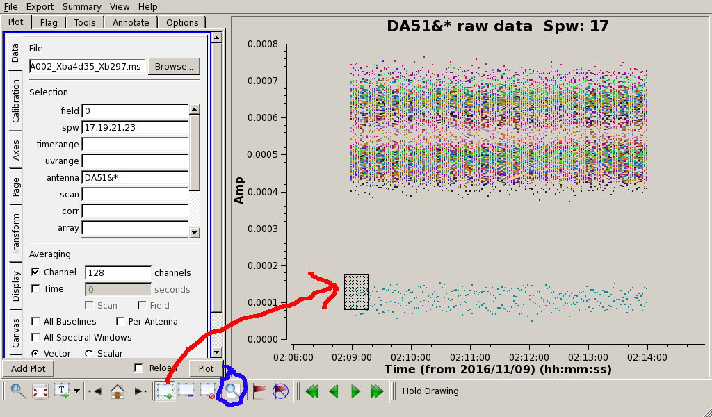
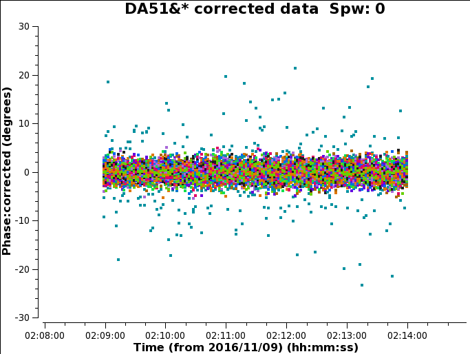
Because this is an entire antenna, and it could just be a mis-scaling (gains are not completely zero) you might want to continue calibration and examine after applying amplitude and phase corrections. In fact, this shows that DV04 is still much noisier in amplitude and phase.So, I inserted a flagging comand in the script, see Step 10 below.
Back in the script, steps 9 and 10 produce another listing of the split data file, 'uid___A002_Xba4d35_Xb297.ms.split', and applies flags such as for shadowing and the edge channels of each spw. Here is the extra flag command due to DV04 being bad
  flagdata(vis = 'uid___A002_Xba4d35_Xb297.ms.split',
    mode = 'manual',
    antenna='DV04',
    flagbackup = False)
Step 11 sets the flux density of the QSO used as a standard. This is a 'grid source', a group of compact QSO monitored every few weeks, along with a primary standard such as Neptune. The most accurate flux density is derived by fitting across a few measurements so it may be updated shortly after observations are taken. The accuracy is a few percent (see technical handbook).
setjy(vis = 'uid___A002_Xba4d35_Xb297.ms.split',
    standard = 'manual',
    field = 'J0238+1636',
    fluxdensity = [0.843698500354, 0, 0, 0],    # flux density (Jy) at reffreq
    spix = -0.530819508421,                     # spectral index
    reffreq = '343.97895GHz')
Step 12 saves the current flagging state, as the calibration tasks can flag more data (which you might want to undo).
 flagmanager(vis = 'uid___A002_Xba4d35_Xb297.ms.split',
    mode = 'save',
    versionname = 'BeforeBandpassCalibration')    # name chosen by user
Execute these steps:
mysteps=[9,10,11,12]
 execfile('uid___A002_Xba4d35_Xb297.ms.scriptForCalibration.py')
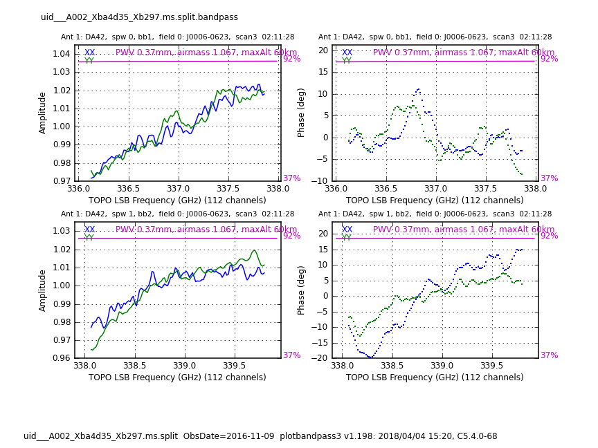
Step 13 leads to the creation of a bandpass table. To start with, for the BP calibrator, the channels are averaged in order to derive preliminary phase corrections as a function of time. This requires combining channels with uncorrected phase, so there is some decorrelation, but the time-dependent corrections are good enough to apply to the data to allow the BP calibrator data to be averaged in time to give enough S/N to derive corrections as a function of frequency in each narrow spectral channel, i.e. the bandpass table.
 gaincal(vis = 'uid___A002_Xba4d35_Xb297.ms.split',
    caltable = 'uid___A002_Xba4d35_Xb297.ms.split.ap_pre_bandpass', # output cal table phase-time
    field = '0', # J0006-0623                                # select bandpass calibrator
    spw = '0:0~127,1:0~127,2:0~127,3:0~127',
    scan = '1,3',
    solint = 'int',                                          # one solution per integration
    refant = 'DA51',
    calmode = 'p')                                           # phase-only solutions

bandpass(vis = 'uid___A002_Xba4d35_Xb297.ms.split',
    caltable = 'uid___A002_Xba4d35_Xb297.ms.split.bandpass', # output BP table (a&p-time)
    field = '0', # J0006-0623
    scan = '1,3',
    solint = 'inf',                                          # combine all times within a scan
    combine = 'scan',                                        # ... and combine all scans
    refant = 'DA51',
    solnorm = True,                                          # normalise amp gains
    bandtype = 'B',                                          # Solve pols XX, YY separately
    gaintable = 'uid___A002_Xba4d35_Xb297.ms.split.ap_pre_bandpass') # apply phase-time cal table
mysteps=[13]
 execfile('uid___A002_Xba4d35_Xb297.ms.scriptForCalibration.py')
The flux scale has not yet been applied to these data so the bandpass amplitude solutions, shown below for 2 spw of one antenna, are normalised.
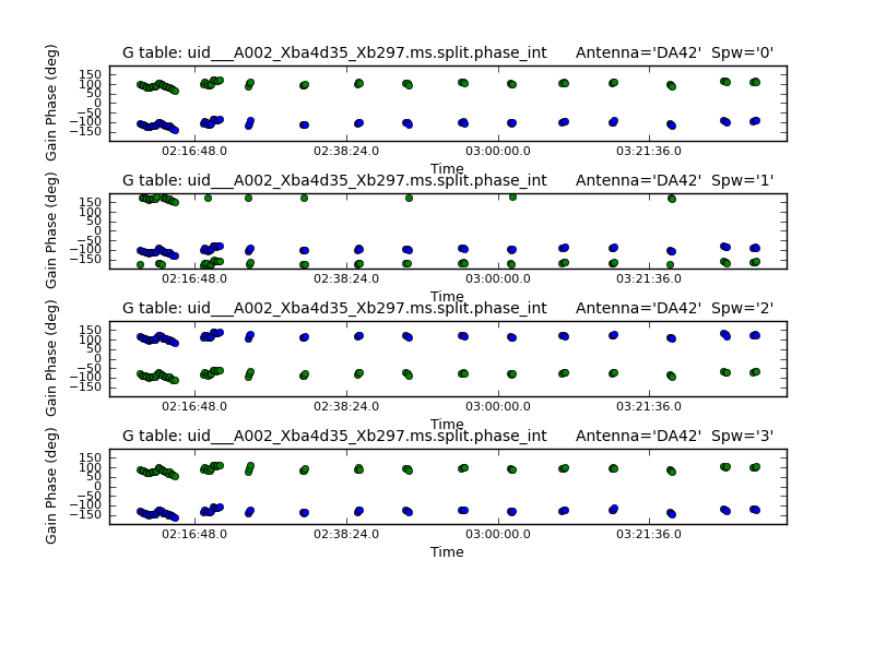
Step 15 derives phase and amplitude solutions as a function of time (i) for all calibration sources, to establish a flux scale; (ii) in order to derive corrections from the phase reference source to apply to the target.
The first gaincal uses per-integration solutions for phase; all these calibration sources have high S/N and are known to be pointlike, so that gives the most accurate solutions.
 os.system('rm -rf uid___A002_Xba4d35_Xb297.ms.split.phase_int')
  gaincal(vis = 'uid___A002_Xba4d35_Xb297.ms.split',
    caltable = 'uid___A002_Xba4d35_Xb297.ms.split.phase_int',
    field = '0~1,3~3', # J0006-0623,J0238+1636,J0217-0820
    solint = 'int',
    refant = 'DA51',
    gaintype = 'G',                       # separate solutions for XX and YY
    calmode = 'p',
    gaintable = 'uid___A002_Xba4d35_Xb297.ms.split.bandpass') # apply bandpass calibration
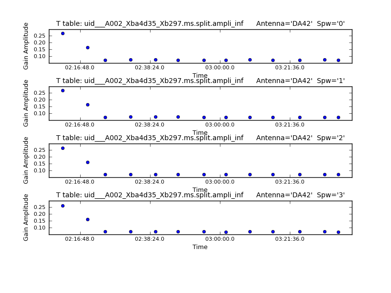
Next, amplitude solutions are derived per-scan, with more averaging. Amplitude errors are usually slower-changing in time. Also, we assume that both polarizations are affected equally and since we are only using a total-intensity model and don't need to calibrate for polarization, we combine the polarizations.
 os.system('rm -rf uid___A002_Xba4d35_Xb297.ms.split.ampli_inf')
  gaincal(vis = 'uid___A002_Xba4d35_Xb297.ms.split',
    caltable = 'uid___A002_Xba4d35_Xb297.ms.split.ampli_inf',
    field = '0~1,3~3', # J0006-0623,J0238+1636,J0217-0820
    solint = 'inf',                       # average in time up to each scan boundary
    refant = 'DA51',
    gaintype = 'T',                       # combine XX and YY
    calmode = 'a',
    gaintable = ['uid___A002_Xba4d35_Xb297.ms.split.bandpass', 'uid___A002_Xba4d35_Xb297.ms.split.phase_int'])
                                          # apply bandpass and per-integration phase solutions
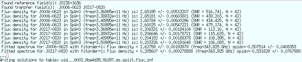
In the next stage, task fluxscale is used to compare the raw flux measurements (correlations) with the flux for the known source which we set as a model with setjy. This produces a log file with the results which are also written to a python dictionary fluxscaleDict (this is a handy facility for any task which produces measurements) and also scales the input calibration table so that the correction factors, when applied, will scale the amplitudes in Jy as well as correcting temporal fluctuations.
  os.system('rm -rf uid___A002_Xba4d35_Xb297.ms.split.flux_inf')
  os.system('rm -rf uid___A002_Xba4d35_Xb297.ms.split.fluxscale')
  mylogfile = casalog.logfile()
  casalog.setlogfile('uid___A002_Xba4d35_Xb297.ms.split.fluxscale')

  fluxscaleDict = fluxscale(vis = 'uid___A002_Xba4d35_Xb297.ms.split',
    caltable = 'uid___A002_Xba4d35_Xb297.ms.split.ampli_inf', # input gain table
    fluxtable = 'uid___A002_Xba4d35_Xb297.ms.split.flux_inf', # scaled gain table
    reference = '1') # J0238+1636
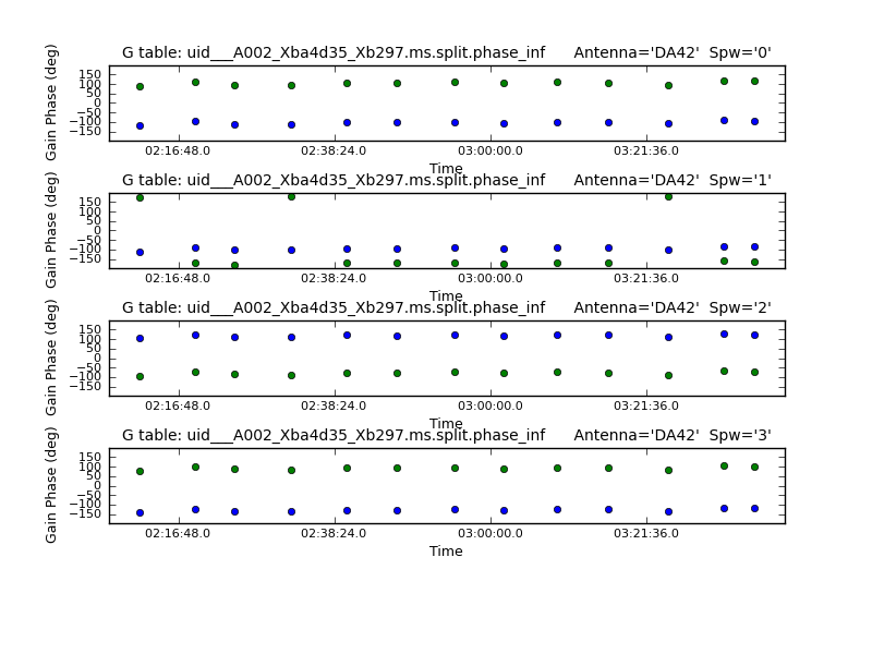
In the last part of this step, another phase-solution table is made with per-scan solutions in order to get better S/N to interpolate over the target.
 casalog.setlogfile(mylogfile)
os.system('rm -rf uid___A002_Xba4d35_Xb297.ms.split.phase_inf')
 gaincal(vis = 'uid___A002_Xba4d35_Xb297.ms.split',
 caltable = 'uid___A002_Xba4d35_Xb297.ms.split.phase_inf',
 field = '0~1,3~3', # J0006-0623,J0238+1636,J0217-0820
 solint = 'inf',
 refant = 'DA51',
 gaintype = 'G',
 calmode = 'p',
 gaintable = 'uid___A002_Xba4d35_Xb297.ms.split.bandpass')
These plots show the phase solutions per integration and per scan, for one antenna, and the per-scan amp solutions (before fluxscale). Part of the fluxscale log is also shown.
Run this step after step 14, which saves the flagging state:
mysteps=[14,15]
 execfile('uid___A002_Xba4d35_Xb297.ms.scriptForCalibration.py')
After saving the flags again, step 17 applies the calibration. The per-integration phase solutions are applied to the bandpass and flux scale calibrator and the per-scan solutions to the target and the phase-ref (in order to compare with the target, if you wish).
  for i in ['0', '1']: # J0006-0623,J0238+1636
    applycal(vis = 'uid___A002_Xba4d35_Xb297.ms.split',
      field = str(i),
      gaintable = ['uid___A002_Xba4d35_Xb297.ms.split.bandpass', 'uid___A002_Xba4d35_Xb297.ms.split.phase_int', 'uid___A002_Xba4d35_Xb297.ms.split.flux_inf'],
      gainfield = ['', i, i],
      interp = 'linear,linear',
      calwt = True,
      flagbackup = False)
  applycal(vis = 'uid___A002_Xba4d35_Xb297.ms.split',
    field = '3,4~48',                            # phase-ref, target fields
    gaintable = ['uid___A002_Xba4d35_Xb297.ms.split.bandpass', 'uid___A002_Xba4d35_Xb297.ms.split.phase_inf', 'uid___A002_Xba4d35_Xb297.ms.split.flux_inf'],
    gainfield = ['', '3', '3'], # J0217-0820     # use solutions from source 3, i.e. the phase-ref, for the time-dependent solutions
    interp = 'linear,linear',
    calwt = True,
    flagbackup = False)
Finally the science data are split out and flags saved again
mysteps=[16,17,18,19]
 execfile('uid___A002_Xba4d35_Xb297.ms.scriptForCalibration.py')
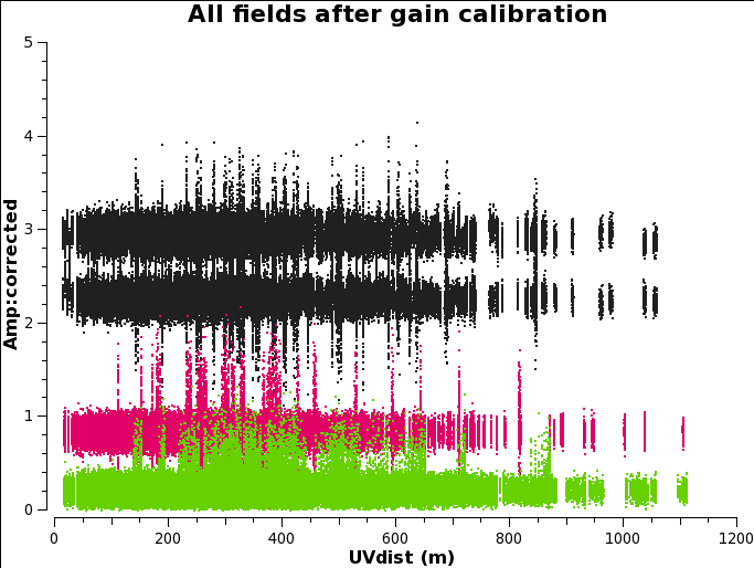
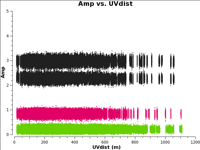
This shows calibrator amplitudes (each in a different colour) as a function of uv distance, from my first attempt and after this execution with DVO4 flagged.
This will give you a file called uid___A002_Xba4d35_Xb297.ms.split.cal which is ready for imaging, see Simple Continuum Imaging